ML Madness

March Madness brings about spirited competition amongst friends and family to see who can pick the better basketball tournament bracket. Some pick theirs randomly, some pick by favorite mascot, while others try to use in-depth basketball knowledge to get the edge. At the end of the day, however, there is one winner and many losers.

To add to the competitive atmosphere I decided to pit a bunch of machine learning algorithms against each other to see which could generate the better bracket. In this post I detail a methodology for collecting college basketball data, training ML models to predict game outcomes, and filling out brackets for tournaments to come. The entirety of the code used can be found here. Since I am posting this before the tournament starts I will come back in April and revisit how the models performed.

• Data Collection
• Predicting Outcomes
• Results
  • Brackets
• Real Life Performance
• Conclusion and Points of Improvement

Data Collection

There are a number of college basketball datasets already available online, which makes the data collection straightforward. This dataset contains NCAA tournament results dating back to 1985 (when the tournament was expanded to 64 teams). Additionally, this site displays end-of-season statistics for every team from 2008 to 2022. Both of the above datasets can be directly downloaded as CSVs. I do this in Python and left join the two CSVs along year and team.

Predicting Outcomes

The ML problem is set up to predict the winner of a game based on information about the two teams playing. In this setup the model is given

and predicts a 1 if \(\textrm{team }1\) wins and a 0 if \(\textrm{team }2\) wins. The first 3 features and the output label are all available from the tournament results dataset. The rest are taken from the end-of-season statistics dataset. This contains the following statistics for each team, each year: Conference, Games Played, Games Won, Adjusted Offensive Efficiency, Adjusted Defensive Efficiency, Power Rating, Effective Field Goal Percentage Shot, Effective Field Goal Percentage Allowed, Turnover Rate, Steal Rate, Offensive Rebound Rate, Offensive Rebound Rate Allowed, Free Throw Rate, Free Throw Rate Allowed, 2Pt %, 2Pt % Allowed, 3Pt %, 3Pt % Allowed, and Adjusted Tempo.

See the columns on the dataset’s website for more information on what these mean. Each of these stats are taken from both teams and inputted into the model. Each of these columns are normalized in the final dataset.

To rapidly try out many different models I used those already available in sklearn. A subset of the classification models were fit on the above training data. Grid search was used to find good hyperparameters for each model. Then 5-fold cross-validation was used to score each model based on average accuracy.

Results

After tuning and fitting each model the best accuracy was achieved with the Support Vector Machine (SVM) classifier at 72%. The accuracies for each model are shown below.

72% is not great, but it is still better than the random guessing model. Also given that we are just using a couple end-of-season statistics this seems like a reasonable accuracy. Better predictions would probably require more sophisticated input data.

Brackets

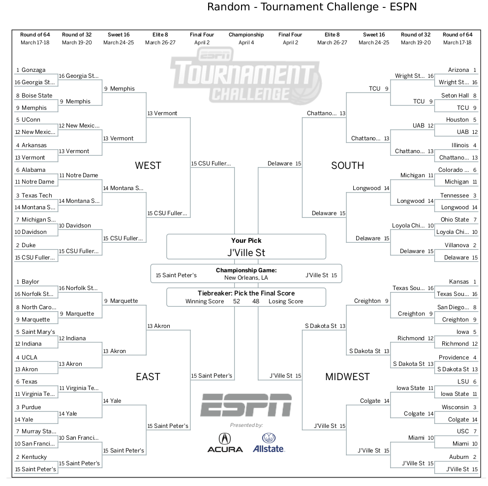
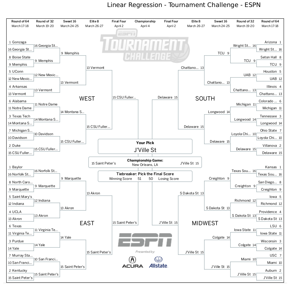
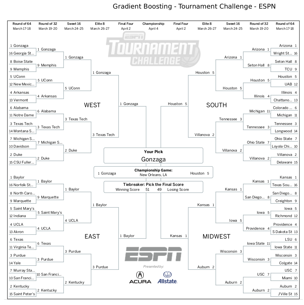
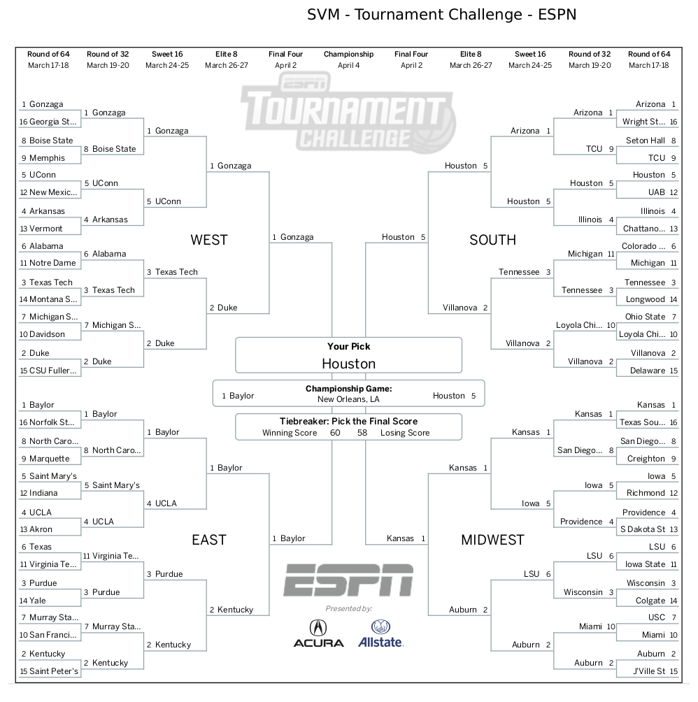
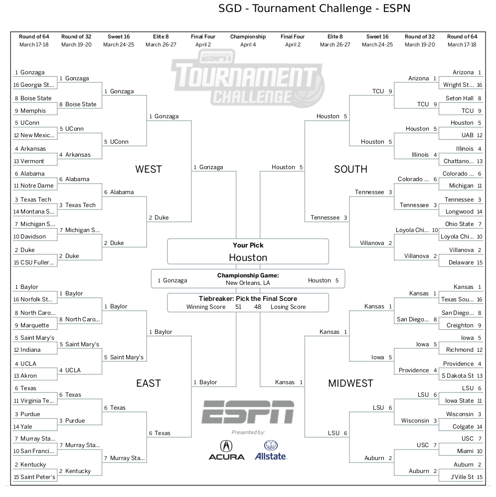
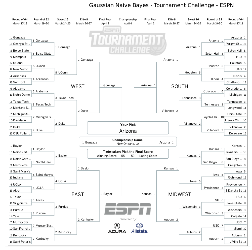
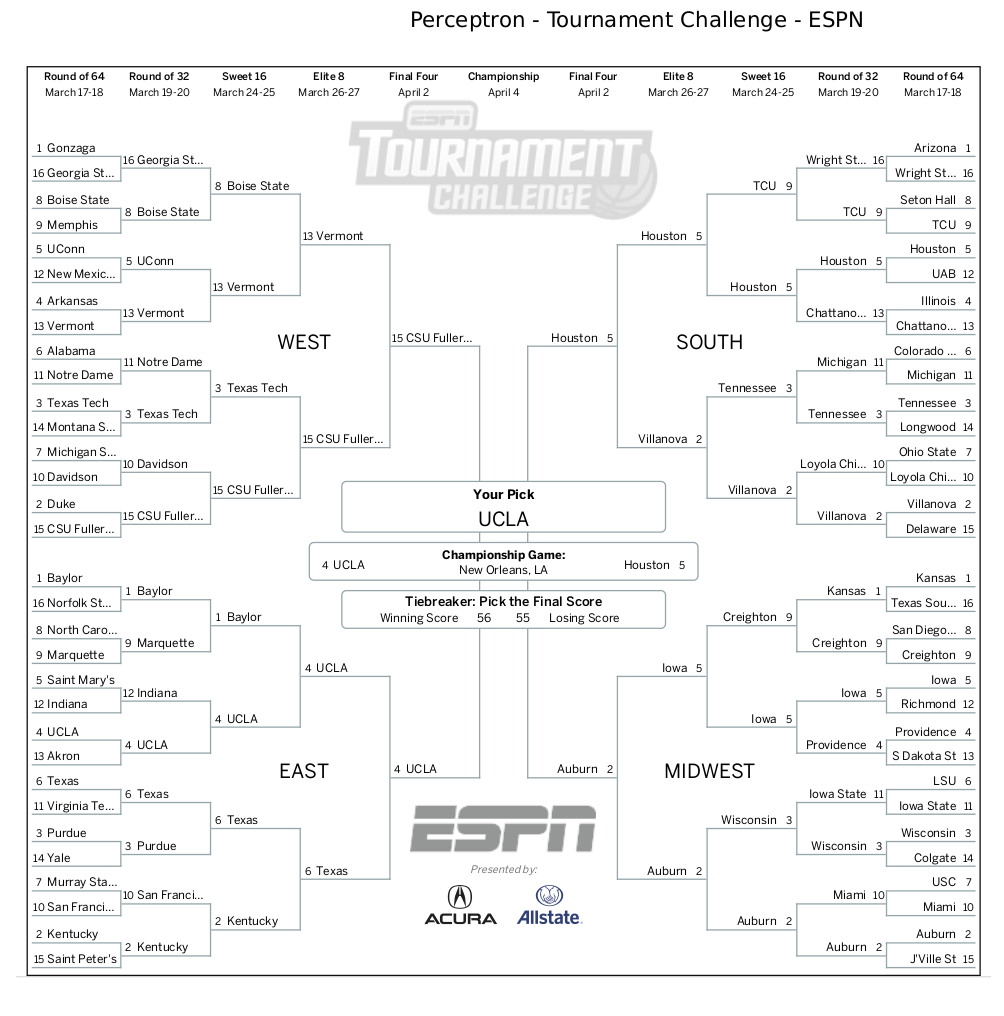
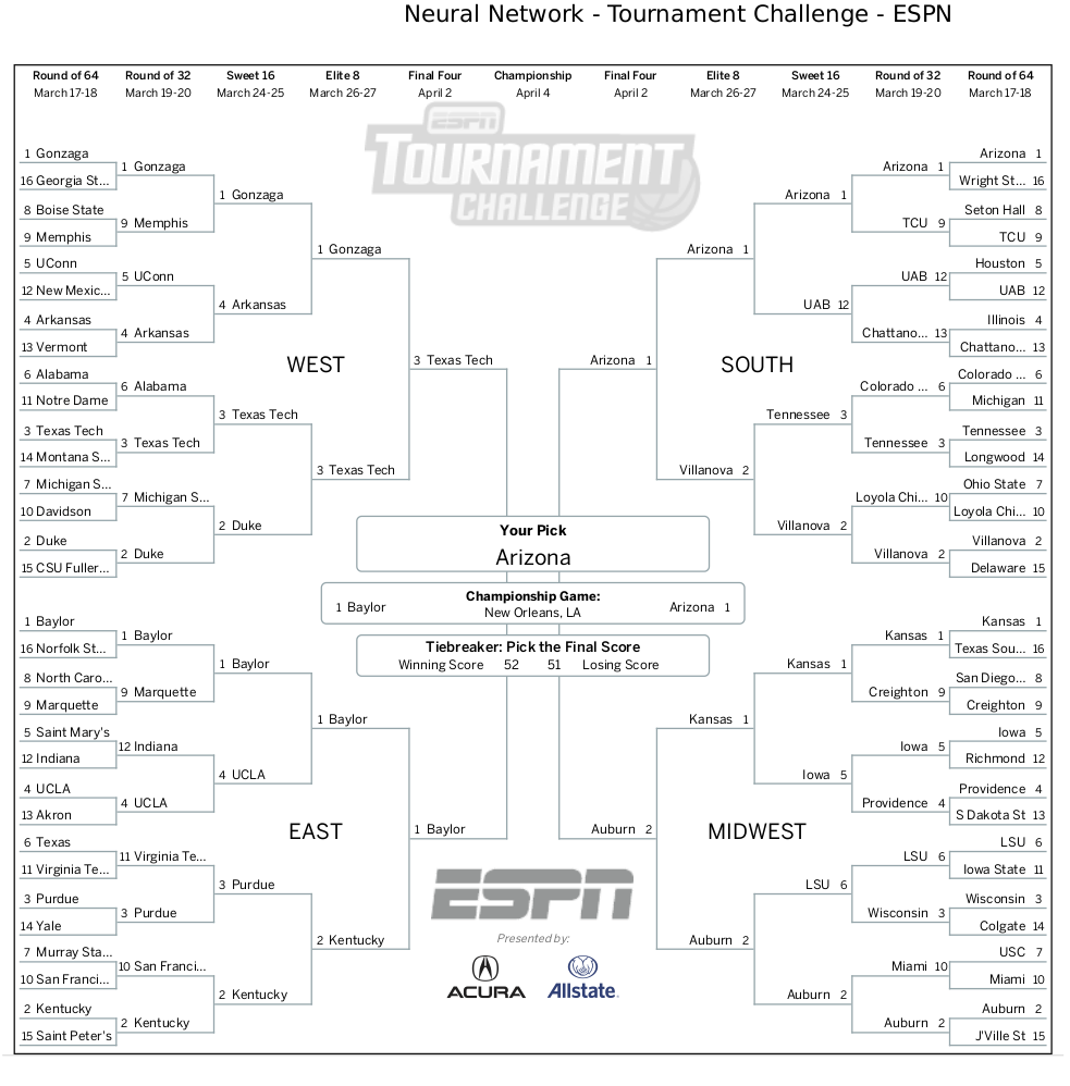
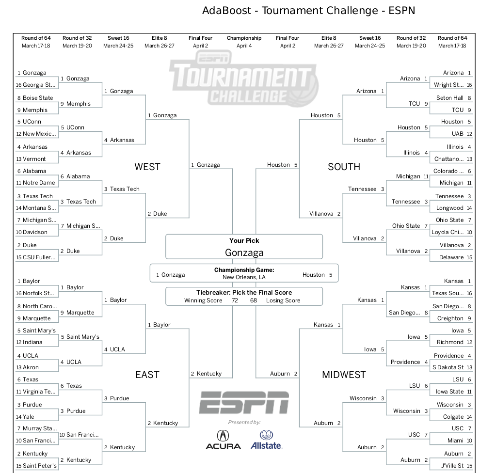
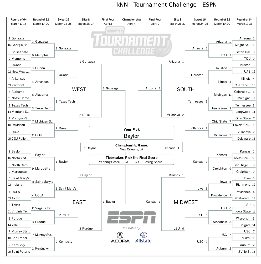
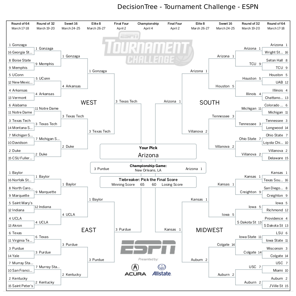
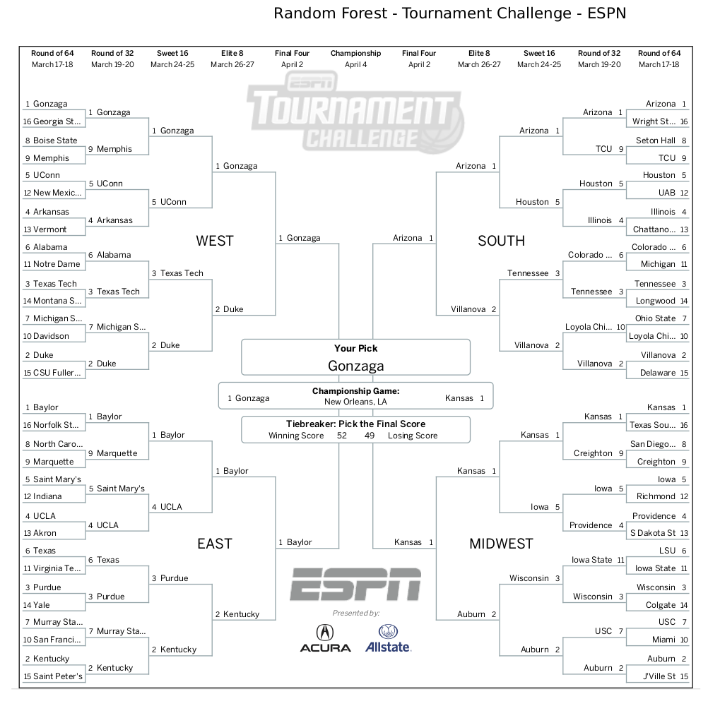
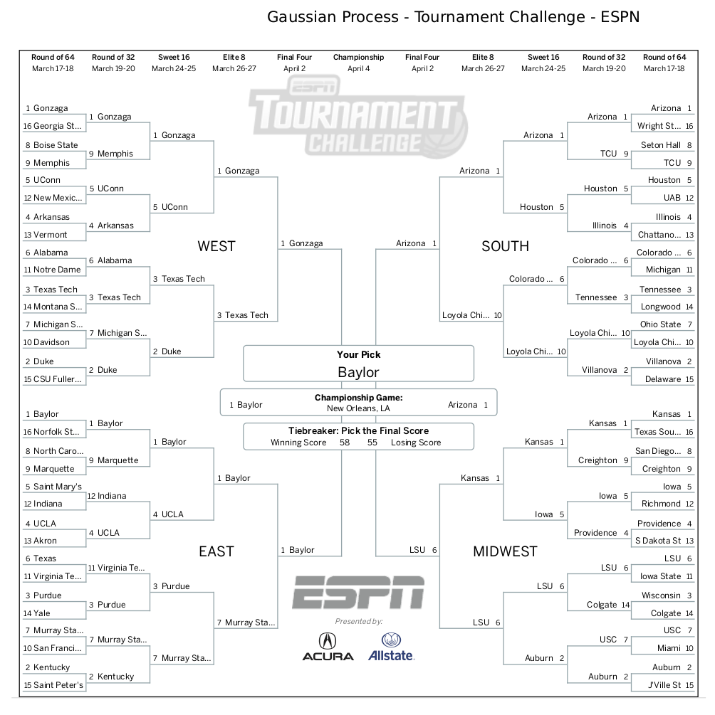
I simulated the 2022 tournament using each of the trained models. I inputted each generated bracket into ESPN’s bracket challenge and put screenshots of the resulting brackets below. Also included is my personal bracket, which will serve as a comparison point to the ML generated brackets.

Previous Next

Real Life Performance

Here are the scores of each bracket at the end of the tournament. The second plot shows the percentile of the bracket within the national pool.

Random Forest classifier wins! With a score of 780 it finished in the 87.2 percentile nationwide. Interestingly this model did not have the highest testing accuracy. The model with the highest accuracy on the training data, the SVM, came in 2nd overall landing in the 75.9 percentile.

Ultimately none of the brackets picked Kansas as the winner. The Random Forest had Kansas in the championship game, which is why it ended up scoring the highest. Additionally, none of them predicted the magic Saint Peter’s run, albeit, neither did most of the country.

Conclusion and Points of Improvement

The results were decent and go to show the amount of unpredictability in the NCAA tournament. However, they are very informative and give me some ideas for how to improve by next March.

First, all of the brackets scored very low due to performing poor in the later rounds. There were lots of upsets early on, but traditionally good teams ended up surviving into the final games. This hurt the final score of most of the models, since games are weighted by round such that each round of the tournament contributes equally to the final tally. Obviously predicting later games is difficult, but I can try to bias the models towards them. One trivial way to do this is to train to optimize bracket score instead of game outcome prediction rate.

Second, there are many important statistics left out of my model. For instance the KenPom scores could also be informative inputs into the model. Next year I will scrape more statistics to use as inputs into the model. Related to this is historical information about the teams. This year we saw all “blue-bloods” in the final four. Historically good teams, despite their statistics, are still favored to make it far in the tournament.

Finally, time series data can be included to help account for momentum. Sometimes teams get “hot” at the end of their season and come into the tournament with considerable momentum. Their early season statistics may skew the aggregate statistics enough to confuse the model. Using time series models such as LSTM neural networks may ameliorate final results.

Altogether, the experiment was fun to follow along throughout March and now I have an extremely “scientific” means to validate my future ML model selections. Next year I will be back with some hopefully improved models.