Code Art

A fun hobby of mine is trying to create art with code. I am quite poor at the standard approach to art, so I am fond of using what I am good at to create aesthetically pleasing things. It is also fun to just try random things and see what pops out. I particularly appreciate techniques, which expose structure unexpectedly. One example of this is writing functions for red, green, and blue, which take a pixel coordinate and map it to a color value. Just this simple method can create some beautiful and quite unexpected images.

I made this website here, which allows custom code art generation in your browser. It is what I use to generate all the below samples. Check out the Preset selection to see some already made art. It is entirely javascript based so feel free to clone the source and just run it locally.

• Mandelbrot
• Hearts
• Trig Functions
• Sierpinski Triangles
• Alternative Color Models
• Coffee Stains

Rainbow

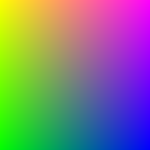
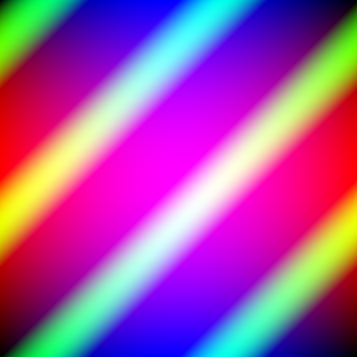
The easiest and most simple example is a color gradient. We can linearly interpolate each color channel from edge to edge. For instance,

red(i, j, width, height) {
  return 255 * (height - i)/height;
}
green(i, j, width, height) {
  return 255 * (width - j)/width;
}
blue(i, j, width, height) {
  return 255 * j/width;
}

This gives use the nice color gradient shown below.

Mandelbrot

While seemingly complex, the Mandelbrot Set maps quite nicely to this process. The Mandelbrot Set is centered around a complex series \(z_{n+1} = z_n^2 + c\), where \(z,c \in \mathbb{C}\). Given a complex number \(c\) and \(z_0 = 0\), if \(z_n\) remains bounded as \(n\) tends towards infinity, then \(c\) is in the Mandelbrot Set. If \(z_n\) diverges towards infinity, then \(c\) is not in the Mandelbrot Set.

Since complex numbers are coordinates in a 2D plane, this maps exceedingly well to our pixel generation method. For any given pixel \((row, column)\), if \(c = row + i\cdot column\) remains bounded, then draw black. Otherwise draw white at that pixel. This gives a nice rendering of the Mandelbrot Set. We can also use the number of iterations it took to diverge to determine how to shade the pixel color.

red(i, j, width, height) {
  let x0 = (j / width) * 3 - 2;
  let y0 = ((height-i) / height) * 2.0 - 1.0;
  let x = 0, y = 0, iter = 0, max_iter = 100;

  while (x*x + y*y <= 4 && iter < max_iter) {
    let tmp = x*x - y*y + x0;
    y = 2*x*y + y0;
    x = tmp;
    iter += 1;
  }

  let scaled_color = Math.pow((iter / max_iter), 0.25) * 255;
  return scaled_color;
}
green(i, j, width, height) {
  let x0 = (j / width) * 3 - 2;
  let y0 = ((height-i) / height) * 2.0 - 1.0;
  let x = 0, y = 0, iter = 0, max_iter = 100;

  while (x*x + y*y <= 4 && iter < max_iter) {
    let tmp = x*x - y*y + x0;
    y = 2*x*y + y0;
    x = tmp;
    iter += 1;
  }

  let scaled_color = Math.pow((iter / max_iter), 0.25) * 255;
  return scaled_color;
}
blue(i, j, width, height) {
  return 255;
}

This code gives us the following rendering:

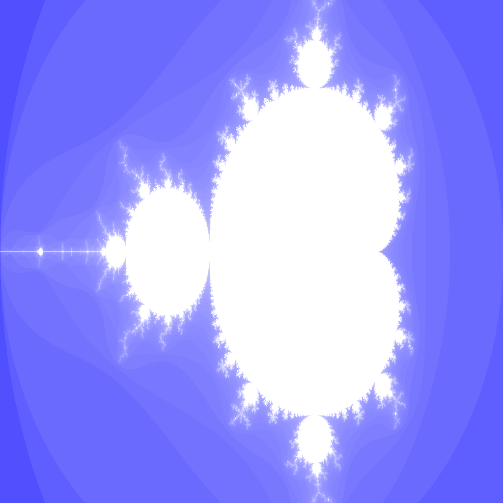
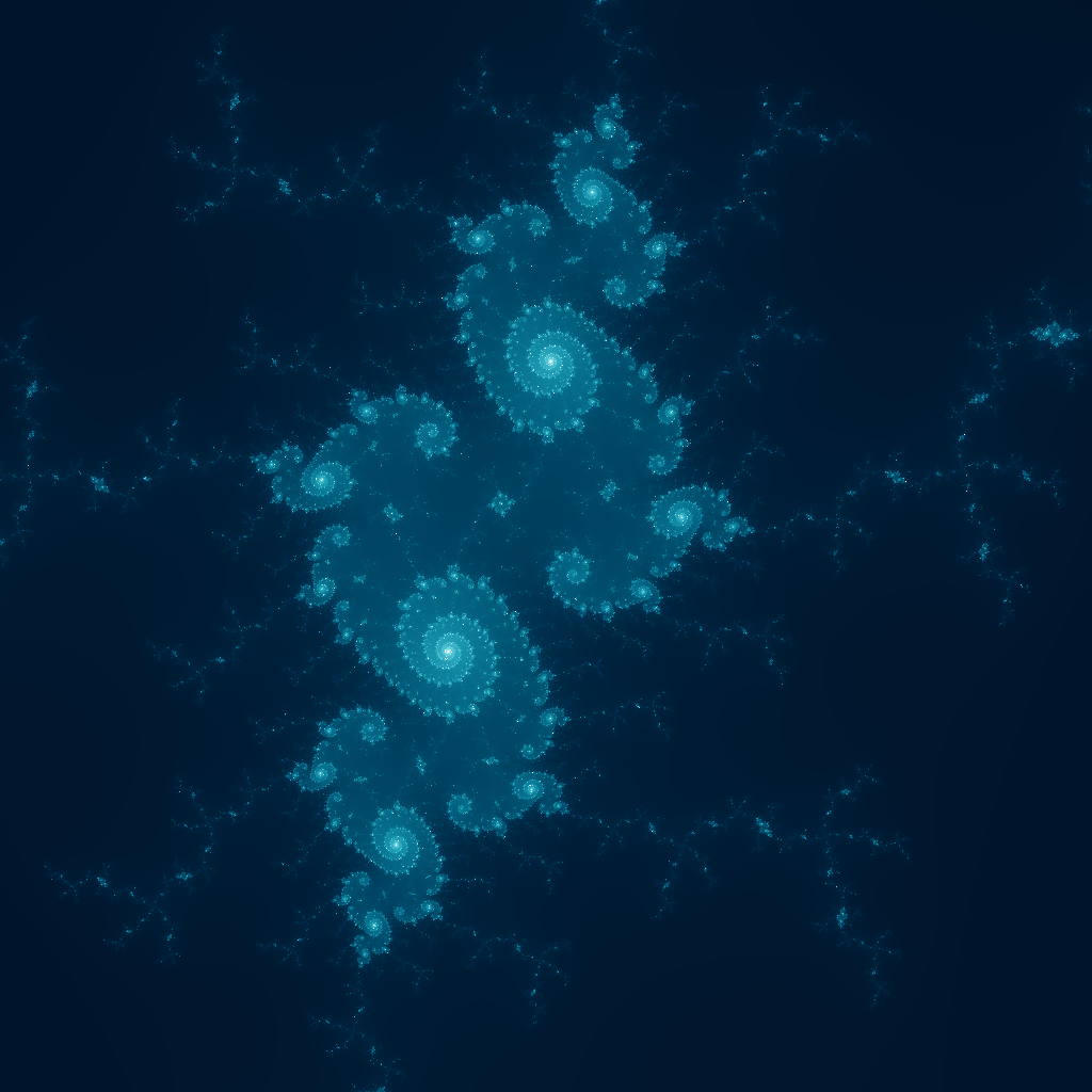
However, we can use Hue, Saturation, Value (HSV) color channels to color the image for more color. See the code here.

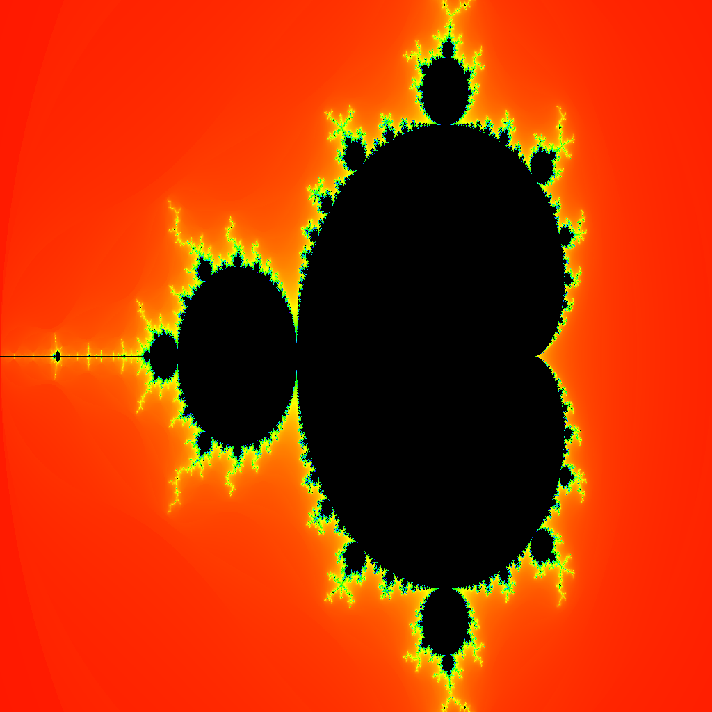
We can also zoom on different sections of the set to get pretty renderings (inspired by this post).

Hearts

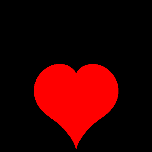
Likewise, any curve can be mapped into this pixel space. Take for instance, \(r(\theta) = 2 - 2\sin\theta + \sin\theta \frac{\sqrt{\lvert \cos\theta \rvert}}{\sin\theta + 1.4}\).

To plot this we need to first map our i,j from pixel-space to coordinate space. This can be done by \(x = (j / width) * (max - min) + min\) and \(y = ((height - i)/height) * (max - min) + min\). Now we have an \(x\) and \(y\) and we know that \(r = \sqrt{x^2 + y^2}\), \(\sin\theta = \frac{y}{r}\), and \(\cos\theta = \frac{x}{r}\). After calculating \((r, \sin\theta, \cos\theta)\) for a pixel \((i, j)\) you can determine the color of that pixel based on the result of \(r < 2 - 2\sin\theta + \sin\theta \frac{\sqrt{\lvert \cos\theta \rvert}}{\sin\theta + 1.4}\). If true, then color the pixel, otherwise don’t.

This is fairly straightforward to translate to code and it gives us a nice big heart:

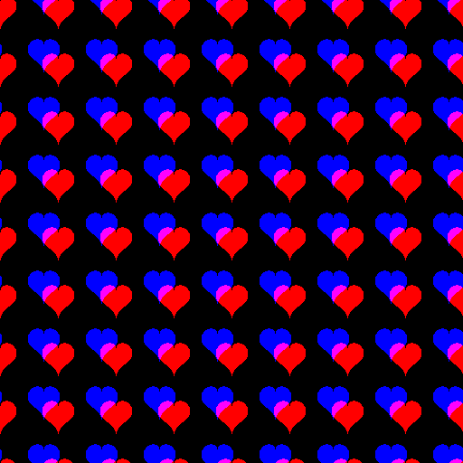
You can make this a pattern by offsetting \(x\) and \(y\) by \(round(x/8)*8\) and \(round(y/8)*8\), respectively. This gives a nice grid pattern. See the code here.

Trig Functions

Another use of this style of code art is visualizing mathematical phenomena in a visually appealing manner. For example, consider the trig functions and their uses in physical applications. Perhaps the simplest of uses is in modeling waves and frequencies. Here we have several properties: period(\(\frac{2\pi}{\omega}\)), amplitude(\(A\)), phase shift(\(\varphi\)) and vertical shift(\(B\)). See below,

This can map to the color values of the picture to produce nice gradient values. For instance, if we calculate red as

then we get a nice “red wave” from top to bottom. Here the amplitude is 255, because color values belong in \([0, 255]\). The wavelength is the full height of the image and the varying parameter, \(i\), runs from the top to the bottom of the image. This gives the nice gradient effect from top-to-bottom seen below.

We can build on top of this and add a blue wave in the horizontal direction. Finally, adding green waves at higher frequency in the diagonal (\(i + j\)) direction gives us the below image. See the code here.

Sierpinski Triangles

Sierpinski Triangles are another example of a fractal. It consists of a pattern of self-repeating triangles.

One way to draw Sierpinski triangles is with turtle graphics and recursion. For every triangle you draw its 3 sub-triangles and continue this recursive pattern until you meet some threshold or triangle depth limit. While an interesting application of recursion, it lacks the wow factor due to its blatant structure. Drawing triangles gives triangles. No big surprises there.

However, there is a particularly neat way to draw Sierpinski triangles using combinatorics and some bitwise operations that is completely surprising.

The first important observation, and the crux of this method, is that Pascal’s triangle modulo 2 is the Sierpinski triangle. Pascal’s triangle has 1s along its edges and each interior number is the sum of the two numbers above it.

            1                                     0
          1   1                                 0   0
        1   2   1               =>            0   1   0
      1   3   3   1                         0   0   0   0
    1   4   6   4   1                     0   1   1   1   0
  1   5   10  10  5   1                 0   0   1   1   0   0

The triangle on the right gives an example of the triangle modulo 2. Notice that the zeroes form a Sierpinski triangle. The pattern becomes even more evident with more rows.

So what does this have to do with drawing pixels to the screen? To see how one must first understand the relationship between Pascal’s triangle and binomial coefficients. Each element of the triangle, at row \(n\), column \(k\), can be expressed using the binomial coefficient \(\binom{n}{k}\).

Therefore, each element of the triangle on the right can be calculated as \(\binom{n}{k} \mod 2\). Now we can map each pixel to a \(k,n\) pair and add color if \(\binom{n}{k} \mod 2\) and no color otherwise. This should render the Sierpinski triangle where \(i < j\).

Now this is great, but we don’t want to compute 3 factorials for every pixel on the screen. Additionally, as soon as the code hits 21! even an unsigned 64 bit integer would overflow, which would required some extra code to support larger numbers. This is do-able, but unnecessary. We can rely on another trick to compute each pixel fast and reliably.

To do this we can use the Lucas Theorem, which states that for a prime \(p\), then

where \(n = n_m p^m + \ldots n_0 p^0\) and \(k = k_m p^m + \ldots k_0 p^0\) are the base-\(p\) expansions of \(n\) and \(k\). This also assumes that \(\binom{n}{k} = 0\) if \(n < k\).

Since in our case \(p = 2\), then \(n_i\) and \(k_i\) can only be zero or one. This means that \(\binom{n_i}{k_i}\) is 0 when \(n_i = 0\) and \(k_i = 1\), otherwise it’s always 1.

Thus we can conclude that \(\binom{n}{k}\) is odd when all of the binary 1 digits of \(k\) are a subset of the ones digits of \(n\). This may not seem much better than computing binomials, but it can be calculated using 3 simple bitwise arithmetic operations.

This leads us to the powerful identity: \(\binom{n}{k} \mod 2 = !( (\sim n) \& k)\), where ! is the NOT operator, ~ is the bitwise NOT operator, and & is bitwise AND operator.

Using the above to color red pixels gives the below Sierpinski triangle.

red(i, j, width, height) {
  return ( !((~i) & j) ) ? 255 : 0;
}

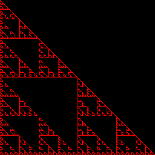
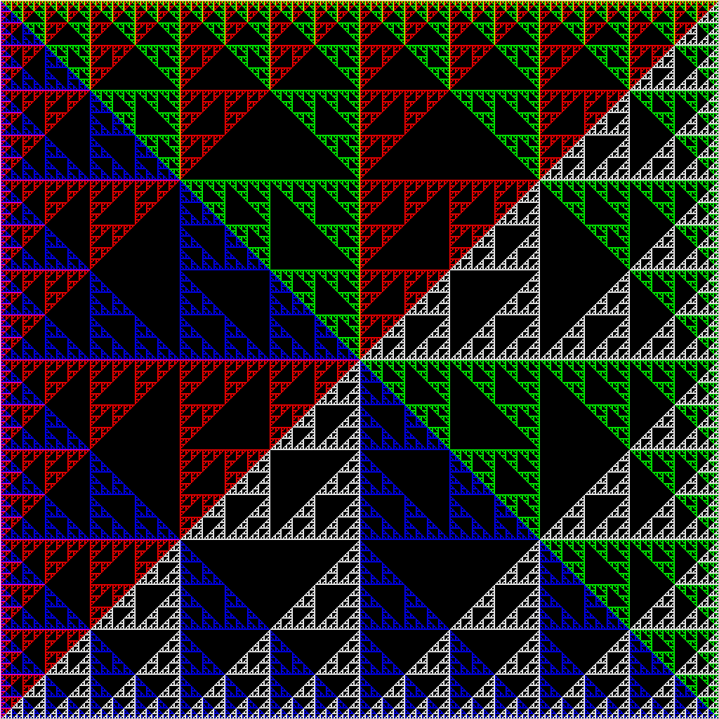
Now flipping the pixels across each axis allows us to superimpose 4 Sierpinski triangles on top of each other in different orientations. See the full code here.

Alternative Color Models

While RGB is fairly straightforward, there are other color models based more on our intuitive understanding of color. For instance, HSL (hue, saturation, lightness) provides a very intuitive basis for constructing colors. Hue values range from 0 to 360, which is a degree providing a base color on the color wheel. Saturation and lightness are percentages providing how saturated and light, respectively, the base color is.

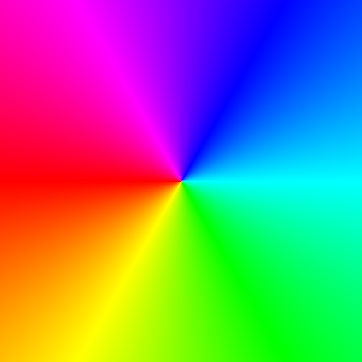
Now using some trig we can reconstruct the hue color wheel.

hue(i, j, width, height) {
  /* map i,j to x,y coordinates centered at middle of image */
  let x = j - width/2, y = height/2 - i;

  /* compute the angle theta in (-pi, pi] of point x,y */
  let t_rad = Math.atan2(y, x);

  /* convert to degrees and map from (-180,180] to (0, 360] */
  return t_rad * 180 / Math.PI + 180;
}

Given constant saturation and lightness of 100% and 50%, this gives the below color wheel.

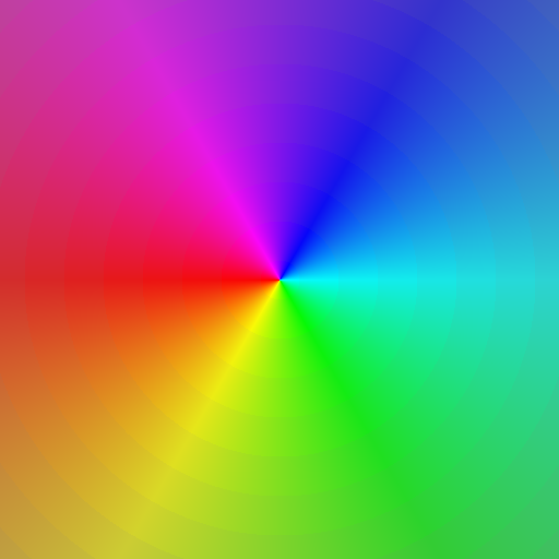
Another added effect is to radially interpolate the saturation of the color and tier the radial bands so the color is more visible.

saturation(i, j, width, height) {
  /* map i,j to x,y coordinates centered at middle of image */
  let x = j - width/2, y = height/2 - i;

  /* find distance from center; max distance is the diagonal */
  let r = Math.sqrt(x*x + y*y);
  let maxR = Math.sqrt(width*width + height*height);

  /* tier the radii to distances of 36 for visual effect */
  r = Math.round(r / 36) * 36;

  /* interpolate the saturation */
  return 100 * (1 - r / maxR);
}

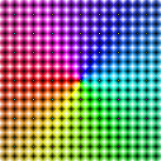
Finally, we have one more color channel to mess with: lightness. Here I construct a grid of points and compute the distance from the current point to the nearest grid point.

lightness(i, j, width, height) {
  /* map i,j to x,y coordinates centered at middle of image */
  let x = j - width/2, y = height/2 - i;

  /* the nearest grid point */
  let disp = 30;
  let cx = Math.round(x / disp) * disp;
  let cy = Math.round(y / disp) * disp;

  /* interpolate lightness between the current point and nearest grid point */
  return (Math.abs(x-cx) + Math.abs(y-cy)) / disp * 100;
}

This gives a cool Collideascope effect.

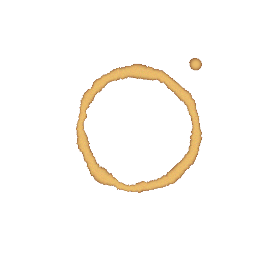
Coffee Stains

Here’s a fun one: can we generate coffee stains using this same method? Sure!

First, we can define two boundaries: the inner and outer edge of the ring of coffee. These we can define using minor and major radii, \(R_{minor}\) and \(R_{major}\), and the parametric curves \(\text{Inner} : (0, 2\pi] \mapsto \mathbb{R}^2\) and \(\text{Outer} : (0, 2\pi] \mapsto \mathbb{R}^2\) defined by

and

If we map pixel coordinate \((i, j) \mapsto (x, y)\), where \((x, y)\) is centered in the middle of the image, then we can use x and y to color the pixel.

First we need the angle \((x, y)\) makes with the origin. Javascript has the \(\text{atan2}\) function, which calculates the arctangent on \([-\pi, \pi)\). Thus, we can get the angle \(\theta\) with \(\theta = \text{atan2}(y, x) + \pi\), which gives \(\theta \in [0, 2\pi)\).

Now that we have the angle of \((x, y)\) within the domain of our functions, we can compute if \(\lVert \text{Inner}(\theta) \rVert_2 < \sqrt{x^2 + y^2} < \lVert \text{Outer}(\theta) \rVert_2\). If true, then color the pixel “coffee colors”, otherwise leave it white.

This seems silly, right? \(\lVert \text{Inner}(\theta) \rVert_2\) is just \(R_{minor}\) and similar for Outer. So why do we need the norm? Why not just use \(R_{minor}\)? We do not just want plain circles. Coffee cups stain with some irregularity. We want to add roughness to the shape to mimic seeping coffee.

We could just let \(A \sim \mathcal{U}[0, a]^2\) and define \(Innner\) as

and similar for \(Outer\), but this would look really jumpy. The radius at 1 radian could differ from the radius at 1.001 and 0.999 radians by up to \(a\), which, across the entire edge of the circle, will look really jumpy. We want a smooth, but still perturbed border. For this we can look at the derivative. Let

and

Now we can define \(A\) using the previous point’s derivative.

where \(B \sim \mathcal{U} [0, a]^2\).

We can choose a satisfiable granularity for \(\epsilon\) when actually calculating the values. The most practical subdivision is by degree. To implement this, we can generate a table before hand with the appropriate adjustments for each value.

Coloring the ring is not too difficult. You can simply interpolate between two shades of brown and add some noise for a nice effect. Using

gives a nice interpolation so that the color can be calculated by \(\text{color} = (\text{light color})\cdot(1 - t) + (\text{dark color})\cdot(t)\). We can also add some noise to the color channels (i.e. some random number less than 10) to give a textured color.

Now we can add a little circle with the same technique around its edge to add a little splash of coffee to the side. This gives us the random coffee spill below.