Reproducing Kernel Hilbert Spaces
Definitions
Hilbert Space: An inner-product space \(\mathcal{H}\) is a Hilbert space if it is also a complete metric space over the metric \(\lVert \bm{x} \rVert = \sqrt{\langle\bm{x},\bm{x}\rangle}\). An inner product space is a vector space for which an inner-product is defined.
Complete Metric Space: A space \(V\) for which every Cauchy sequence in \(V\) has a limit in \(V\). A sequence \(\bm{x}_1, \bm{x}_2, \ldots\) is Cauchy for some metric \(d\) if for all \(r>0\) there exists a positive integer \(N\) such that for all \(m,n > N\) then \(d(\bm{x}_m, \bm{x}_n) < r\). Thus, if a space \(V\) over some metric \(d\) is complete, then all Cauchy sequences \(\bm{x}_1, \bm{x}_2, \ldots\) in \(V\) must have \(M = \lim_{n \to \infty} \bm{x}_n\) such that \(M \in V\).
Reproducing Kernel Hilbert Space: Let \(\mathcal{H}\) be a Hilbert space over real-valued functions defined on some arbitrary set \(\mathcal{X}\). The set of functions on \(\mathcal{X}\) can be considered an inner-product space, since we can define the inner-product of functions \(f(\cdot)\) and \(g(\cdot)\) as
\[\langle f, g \rangle = \sqrt{ \int_{\mathcal{X}} f(\bm x) g(\bm x)\, \mathrm{d}\bm{x}}.\]\(\mathcal{H}\) is a Reproducing Kernel Hilbert Space if there exists a function \(\kappa : \mathcal{X} \times \mathcal{X} \mapsto \mathbb{R}\) with the following two properties:
- \(\kappa (\cdot, \bm x) \in \mathcal{H}\) for all \(\bm{x} \in \mathcal{X}\)
- \(f(\bm x) = \langle f, \kappa(\cdot, \bm x) \rangle_{\mathcal{H}} \quad \forall f \in \mathcal{H} \, \forall \bm x \in \mathcal{X}\) (a.k.a. the reproducing property)
The second property and the nomenclature that \(\kappa\) is called a kernel gives this special space its name.
Feature Map: Let \(\mathcal{H}\) be a Reproducing Kernel Hilbert space (RKHS) associated with a kernel \(\kappa(\cdot, \cdot)\) and some arbitrary set \(\mathcal{X}\). Then the following \(\phi(\bm x)\) is a feature map to the feature space \(\mathcal{H}\)
\[\mathcal{X} \ni \bm x \mapsto \phi(\bm x) \triangleq \kappa(\cdot, \bm x) \in \mathcal{H}\]Notice that \(\phi\) maps vectors to functions. In practice \(\mathcal{H}\) has infinite dimension, so we are mapping points in \(\mathcal{X}\) from finite dimensions to the “much higher” number of infinite dimensions.
Kernel Trick: A popular trick in machine learning is to use the inner product of \(\phi\)’s for feature mapping. \(\bm x, \bm y \in \mathcal{X}\) are mapped to infinite dimensions by \(\phi(\bm x)\) and \(\phi(\bm y)\), but their inner-product
\[\langle \phi(\bm x), \phi(\bm y) \rangle_{\mathcal{H}} = \langle \kappa(\cdot, \bm x), \kappa(\cdot, \bm y) \rangle_{\mathcal{H}} = \kappa(\bm x, \bm y)\]by the reproducing property. Thus, the infinite dimension inner-product of the mappings can be represented by the scalar \(\kappa(\bm x, \bm y) \in \mathbb{R}\).
Positive Definite Kernel: A kernel \(\kappa\) is positive definite if
\[\sum_{n=1}^N \sum_{m=1}^N a_n a_m \kappa(\bm x_n, \bm x_m) \ge 0 \quad \forall a_n,a_m \in \mathbb{R}\]This can also be written as \(\bm{a}^\intercal \mathcal{K} \bm a \ge 0\) where \(\mathcal{K}\) is a matrix such that \(\mathcal{K}_{ij} = \kappa(\bm x_i, \bm x_j)\). Thus, \(\mathcal{K}\) must be positive semi-definite.
Some common examples of positive definite kernels:
- Radial Basis Function (or Gaussian): \(\kappa(\bm x, \bm y) = \exp\left( -\frac{\lVert \bm x - \bm y \rVert^2_2}{2\sigma^2} \right)\)
- Homogeneous Polynomial: \(\kappa(\bm x, \bm y) = (\bm x^\intercal \bm y)^r\)
- Inhomogeneous Polynomial: \(\kappa(\bm x, \bm y) = (\bm x^\intercal \bm y + c)^r\)
- Laplacian: \(\kappa(\bm x, \bm y) = \exp\left(-t \lVert \bm x - \bm y \rVert\right)\)
- Spline: \(\kappa(\bm x, \bm y) = B_{2p+1}\left(\lVert \bm x - \bm y\rVert^2_2\right)\) where \(B_n(\cdot) \triangleq \bigotimes_{i=1}^{n+1} \chi_{[-\frac 1 2, \frac 1 2]} (\cdot)\).
- Sinc: \(\kappa(\bm x, \bm y) = \mathrm{sinc}(\bm x - \bm y)\)
Positive Definite Kernel Functions and RKHS Relationship: Every positive definite kernel \(\kappa : \mathcal{X}\times\mathcal{X} \mapsto \mathbb{R}\) defines a unique RKHS such that \(\kappa(\cdot,\cdot)\) is a reproducing kernel. This goes both ways as well. An RKHS is defined by a unique positive definite kernel.
Representer Theorem: The main reason all this is important. Let \(J : \mathcal{H} \mapsto \mathbb{R}\) be a function defined by
\[J(f) = \sum_{n=1}^{N} \mathcal{L}(y_n, f(\bm x_n)) + \lambda \Omega(\lVert f\rVert)\]where \(f \in \mathcal{H}\), \(\Omega : [0, +\infty] \mapsto \mathbb{R}\) is strictly monotonic increasing, and \(\mathcal{L}:\mathbb{R}^2 \mapsto \mathbb{R}\cup\{\infty\}\). Then the minimization problem
\[f^\star = \argmin_{f\in\mathcal{H}} J(f)\]for some \(\theta_n \in \mathbb{R}\) can be represented by the linear combination
\[f^\star = \sum_{n=1}^{N} \theta_n \kappa(\cdot, \bm x_n)\]This is important because \(J\) can model the empirical loss (or risk) of a statistical prediction model. If \(f(\bm x_n)\) makes some prediction for input \(\bm x_n\) and \(y_n\) is the ground truth, then \(\mathcal{L}(y_n, f(\bm x_n))\) can model the loss of that classification. \(\Omega(\lVert f \rVert)\) exists as a regularization term to keep the complexity of \(f^\star\) lower (i.e. the VC dimension), but we can set \(\lambda = 0\) to avoid this if necessary.
This is tremendously useful for machine learning. Particularly because the minimization problem \(\min_{f}J(f)\) is very difficult. Rather than finding an optimal set of parameters as in traditional statistical models, we are finding an optimal function, which is a difficult problem. This is made even more difficult by the fact that \(\mathcal{H}\) is often an infinite space. Since \(f^\star\) is a linear combination of kernel functions, finding the optimal \(f\) is much easier.
Kernel Support Vector Machines
Support Vector Machines (SVM) provide a very intuitive application of kernels to machine learning. Consider a dataset with 2 classes. Vanilla SVM tries to find a line which divides the two classes with maximum margin between them (wikipedia has good pictures). In higher dimensions it tries to divide the data by a hyperplane. SVM essentially tries to find the line which best divides the data.
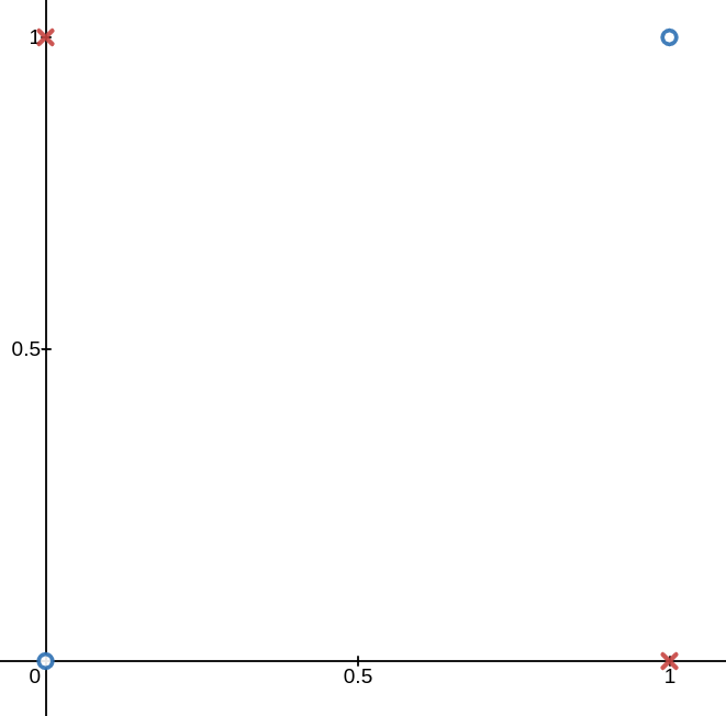
This is very intuitive, but not all data is linearly separable. The de facto example here is the XOR function seen below. No line can divide the blue o’s from the red x’s.
However, if we map the data to a higher dimension using the following mapping
\[\begin{bmatrix} \bm x_1 \\ \bm x_2 \end{bmatrix} \mapsto \begin{bmatrix} \bm x_1 \\ \bm x_2 \\ \bm x_1 \bm x_2 \end{bmatrix}\]then now the data is linearly separable by a plane. So this begs the question: how do we find an optimal set of functions to map \(\bm x\) to a higher dimension? Using Reproducing Kernel Hilbert Spaces of course! In fact by the representer theorem we can map \(\bm x\) to infinite dimensions and model it with finite parameters.
The Wikipedia page on SVMs presents their full theory. Essentially, linear SVM boils down to the following quadratic maximization problem.
\[\begin{aligned} \textrm{maximize} \quad& \sum_{n=1}^N \lambda_n - \frac 1 2 \sum_{n=1}^N \sum_{m=1}^N \lambda_n \lambda_m y_n y_m \bm{x}_n^\intercal \bm{x}_m \\ \textrm{subject to} \quad & 0 \le \lambda_n \le C \\ \quad & \sum_{n=1}^N \lambda_n y_n = 0 \end{aligned}\]However, we want to map \(\bm x \mapsto \phi(\bm x)\) where \(\phi(\bm x) = \kappa(\cdot, \bm x)\). This is the mapping of \(\bm x\) to the higher dimensional feature space. Thus the mapping becomes
\[\begin{aligned} \bm{x}_n^\intercal \bm{x}_m \mapsto & \phi(\bm x_n)^\intercal \phi(\bm x_m) \\ & \kappa(\cdot, \bm x_n)^\intercal \kappa(\cdot, \bm x_m) \\ & \langle \kappa(\cdot, \bm x_n), \kappa(\cdot, \bm x_m) \rangle_{\mathcal{H}} \\ & \kappa(\bm x_n, \bm x_m) \end{aligned}\]and the final cost function in the maximization becomes
\[\sum_{n=1}^N \lambda_n - \frac 1 2 \sum_{n=1}^N \sum_{m=1}^N \lambda_n \lambda_m y_n y_m \kappa(\bm x_n, \bm x_m)\]Now it is clear why the reproducing property of RKHS’s is so helpful. We can map \(\bm x\)’s to infinite dimensional spaces and represent the result using a scalar valued kernel.
Kernel Principal Component Analysis
Principal Component Analysis (PCA) is another good application of kernels. PCA is used as a change of basis for some data \(X \in \mathbb{R}^{n \times m}\) where we have \(n\) data samples each with \(m\) features. We can change the bases of \(X\) in a way such that the covariances between features is maximized. This gives an ideal representation of the data. PCA is typically done by computing the principal component of each feature and projecting each data point using these components. PCA can also be used for dimensionality reduction by only projecting data points by the principal components corresponding to the \(k\) largest eigenvalues. Thus the data would be reduced from \(n\times m\) to \(n\times k\).
Formally, PCA finds a matrix \(W\) that transforms \(X\) with \(X_{\textrm{new}} = XW\). \(w_{(k)}\), the k-th row of \(W\), is calculated as
\[\bm{w}_{(k)} = \argmax_{\bm w} \frac{\bm{w}^\intercal \hat{\Sigma}_k \bm{w}}{\bm{w}^\intercal \bm{w}}\]where \(\hat{\Sigma} = \frac{1}{N} \sum_{n=1}^{N} \bm x_n \bm x_n^\intercal\) is the sample covariance (assuming \(X\) is centered). It can be shown that \(X^\intercal X \propto \hat{\Sigma}\), so we often used \(X^\intercal X\) in the numerator instead. Thus, if we want to reduce the data to \(k\) dimensions, then \(W\) will be the eigenvectors corresponding to the \(k\) largest eigenvalues of \(X^\intercal X\).
This, however, is a linear mapping from \(X\) to \(X_{\textrm{new}}\). What if such a linear data mapping is not ideal? This seems like another great place to utilize RKHS’s and the kernel trick. First define a new sample covariance as
\[\hat{\Sigma}_k = \frac{1}{N} \sum_{n=1}^{N} \phi(\bm x_n) \phi(\bm x_n)^\intercal\]Now it can be shown that \(\hat{\Sigma}\bm u = \lambda \bm u\) has eigenvectors \(\bm u\) in the form of \(\sum_{n=1}^{N} a_n \kappa(\cdot, \bm x_n)\) and thus
\[\mathcal{K}\bm a = N\lambda \bm a\]where \(\bm a = [a_1, \ldots, a_n]^\intercal\) and \(\mathcal{K}_{ij} = \kappa(\bm x_i, \bm x_j)\). Finally, we can project values of \(X\) using the eigenvectors corresponding to the \(k\) largest eigenvalues of \(\mathcal{K}\). In practice we also typically normalize \(\bm a\) such that \(\langle \bm u, \bm u \rangle_{\mathcal{H}} = 1\).
This is a seemingly odd result. We have found better dimensionality reductions by first mapping the data to a higher dimension and then reducing it. However, Kernel PCA outperforms traditional PCA when a linear mapping is not possible. Again the Wikipedia page on Kernel PCA has some good pictures to show this effect.